Flip an Arrow With a Neural Network

Overview

Autoencoders are neural network architectures designed to learn compact representations of data. When trained on images, they compress high-dimensional pixel information into lower-dimensional latent vectors. These latent spaces often capture meaningful structure in the data distribution, forming a continuous manifold where directions correspond to interpretable variations. This property enables controlled modification of image attributes by operating directly in latent space.

In this article we will use Neural Networks to create a latent space for the Arrow Dataset from Kaggle, find concept vector in it and apply it to an arbitrary precedent all using Wolfram Mathematica.

The Arrow Dataset

The arrow dataset comes from Kaggle

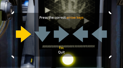
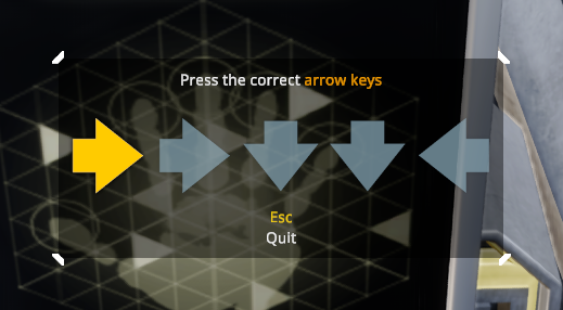
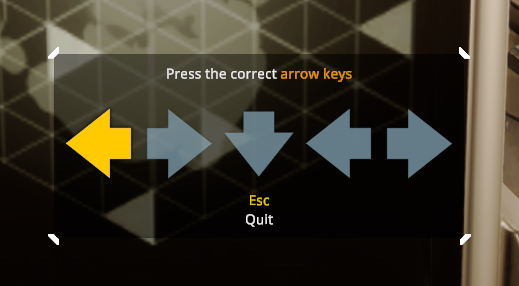
It's a collection of images with arbitrary sequence of arrows in the set {left, right, up, down} recorded during the gameplay of computer game Void Crew.

Autoencoder Structure

An autoencoder consists of two components:

• Encoder: Maps an input image to a latent vector.
• Decoder: Reconstructs an image from a latent vector.

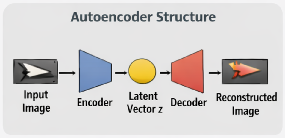
During training, the network learns to minimize reconstruction error. The latent layer becomes a compressed representation that preserves salient features of the input.

Once trained, the decoder can generate new images from arbitrary latent vectors, even those not produced by the encoder. This allows direct exploration of the learned manifold.

In this particular instance the following Autoencode structure was used:

encoder = NetEncoder[{"Image", {414, 94}, "ColorSpace" -> "Grayscale"}];
decoder = NetDecoder[{"Image", "ColorSpace" -> "Grayscale"}];

neckSize = 100;
width = 200;
embeddingNet = NetChain[{
   ConvolutionLayer[width, 3],
   Tanh,
   PoolingLayer[2, 2],
   
   ConvolutionLayer[width, 3],
   Tanh,
   PoolingLayer[2, 2],
   
   ConvolutionLayer[width, 3],
   Tanh,
   PoolingLayer[2, 2],
   
   ConvolutionLayer[width, 3],
   Tanh,
   PoolingLayer[2, 2],
   
   ConvolutionLayer[width, 3],
   Tanh,
   PoolingLayer[2, 2],
   
   FlattenLayer[],
   LinearLayer[neckSize],
   Tanh
   }, "Input" -> {1, 94, 414}]

(*A trick to know what was the last seen shape *)
lastShape = 
  Information[NetExtract[embeddingNet, -3], "InputPorts"]["Input"];
flatSize = 
  Information[NetExtract[embeddingNet, -3], "OutputPorts"]["Output"];

restoreNet = NetChain[{
   LinearLayer[flatSize],
   Tanh,
   ReshapeLayer[lastShape],
   
   ResizeLayer[{Scaled[2], Scaled[2]}, Resampling -> "Nearest"],
   DeconvolutionLayer[width, 3],
   Tanh,
   
   ResizeLayer[{Scaled[2], Scaled[2]}, Resampling -> "Nearest"],
   DeconvolutionLayer[width, 3],
   Tanh,
   
   ResizeLayer[{Scaled[2], Scaled[2]}, Resampling -> "Nearest"],
   DeconvolutionLayer[width, 3],
   Tanh,
   
   ResizeLayer[{Scaled[2], Scaled[2]}, Resampling -> "Nearest"],
   DeconvolutionLayer[width, 3],
   Tanh,
   
   ResizeLayer[{Scaled[2], Scaled[2]}, Resampling -> "Nearest"],
   DeconvolutionLayer[1, 3],
   Tanh
   }, "Input" -> {neckSize}]

Latent Space as a Manifold

The latent space of a trained autoencoder often organizes data along continuous dimensions. Images that are visually similar tend to map to nearby latent vectors. Moving smoothly through latent space typically produces smooth visual transformations in decoded images.

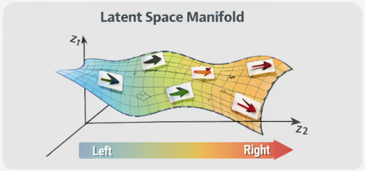
This continuity enables arithmetic operations on latent vectors to produce meaningful changes. Differences between latent vectors can correspond to semantic transformations.

Learning the latent space manifold is equivalent to just training the autoencoder, which can easily be achieved with Wolfram Mathematica's NetTrain:

result = NetTrain[
  NetChain[{embeddingNet, restoreNet}],
  trainData,
  All,
  ValidationSet -> validationData,
  LossFunction -> MeanSquaredLossLayer[],
  TargetDevice -> "GPU",
  WorkingPrecision -> "Real32",
  TimeGoal -> Quantity[60, "Minutes"],
  (*MaxTrainingRounds->2000,*)
  BatchSize -> 16,
  LearningRate -> 0.0001,
  (*Method->{"SGD","Momentum" -> 0.93},*)
  (*TrainingProgressReporting->"Print",*)
  TrainingProgressCheckpointing -> {"Directory", 
    NotebookDirectory[] <> "\\backups", 
    "Interval" -> Quantity[5, "Minutes"]}]
Export[NotebookDirectory[] <> "trainedNet.WLNet", result["TrainedNet"]]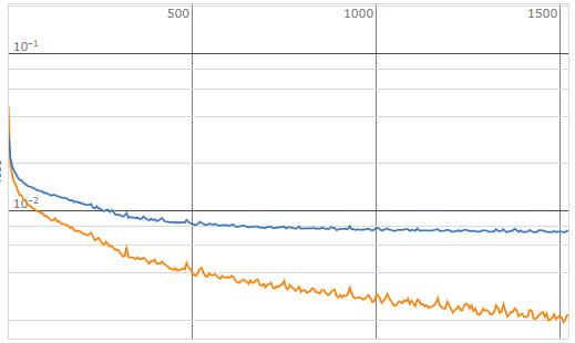

After training the neural network and example of image forwarding through the trained autoencoder may look like this:

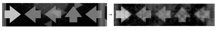
The reconstruction quality leaves much space for improvement, but it will suffice for the demonstration

Concept Vectors in Latent Space

The most interesting property of latent spaces are "concept vectors". A concept vector is constructed by computing the average latent representation of images sharing a common attribute, then subtracting the average latent representation of images without that attribute. The resulting vector approximates a direction in latent space associated with the chosen feature:

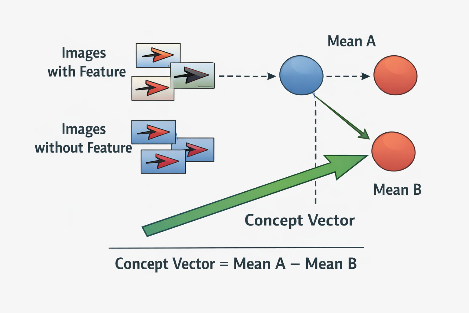
Once a concept vector is identified, it can be added to or subtracted from latent vectors of other images to modify the corresponding feature.

Example workflow:

1. Encode multiple images containing a specific feature.
2. Compute the mean latent vector for these images.
3. Encode images lacking the feature.
4. Compute the mean latent vector for these.
5. Subtract means to obtain a feature direction vector.

Applying this vector to a latent representation modifies the decoded image accordingly.

Here is how that may look on the arrow dataset:

findConcept[labelPattern_]:=Cases[labeledData,HoldPattern[_->labelPattern]]//Keys//Map[embed]//Mean
findConcept[{"right", _, _, _, _}] // unembed
findConcept[{"left",_, _, _, _}] // unembed

Will produce 2 concepts: a concept of leftmost arrow pointing right and a concept of leftmost arrow pointing left:

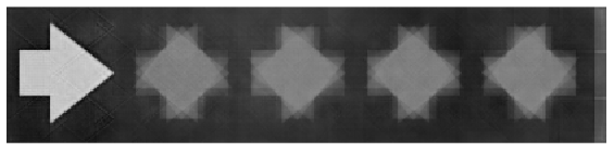
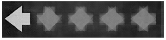
Image Transformation via Latent Vector Arithmetic

Given a latent vector representing an image, adding a scaled concept vector moves the representation along the learned manifold. Decoding the modified vector produces a new image with an adjusted feature.

By varying the magnitude of the added vector, gradual transformations can be generated. This enables smooth rotations, deformations, or style changes without retraining the model or modifying the original image directly.

A trained autoencoder can learn rotational variation if trained on images containing rotated instances of an object. A rotation concept vector can be computed from latent representations of images at different orientations. Adding this vector to the latent representation of a given image yields a decoded image rotated accordingly.

This approach demonstrates that latent spaces can encode geometric transformations as linear directions, even though the underlying image space is highly nonlinear.

Let us apply these ideas. First, find any image with an arrow pointing right and then simply flip the leftmost arrow by moving along the conecpt space into the direction of "left arrow" concept while leaving remaining arrows unchanged:

anyArrowRight=FirstCase[labeledData,HoldPattern[_->{"right",_,_,_,_}]]//First//embed;
Manipulate[unembed[anyArrowRight+x(arrowLeftConcept-arrowRightConcept)],{x,0,1},ContinuousAction->False]

Conclusion

Autoencoder latent spaces form structured manifolds that encode meaningful variations in data. By identifying and applying concept vectors within these spaces, specific features of images can be modified through simple vector operations. This establishes a practical framework for feature-level image manipulation using learned representations rather than direct pixel editing.

The full listing of the wolfram mathematica program is available here.